Neural Networks

FIZ371 - Scientific & Technical Computations | 03/06/2020

Neural Networks

• Introduction

• Comparison of ‘meat’ with ‘silicon’

• Architecture of the neural networks

  • Activity Rule

  • Learning Rule

• Artificial Neural Networks

  • Supervised neural networks

  • Unsupervised neural networks

• Modeling of the neural networks

  • Activity Rule

    • Deterministic

    • Stochastic

• Examples

  • AND gate

  • NOR gate

• Homework #1

• Training a single neuron as a binary classifier

  • ‘Learning by example’

    • Activity Rule

    • Learning Rule

      • The on-line gradient descent algorithm

      • The batch learning algorithm

• Implementation to code

• Code, combined

• Homework #2

• References

• Places of Interest

• Here and then…

Dr. Emre S. Tasci emre.tasci@hacettepe.edu.tr

Introduction

This is how a neuron (nerve cell) looks like: 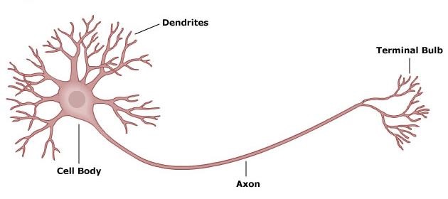Schematics of a neuron Source

We will be referring to this figure a lot but the interesting thing is the fact that computers had been developed long before the understanding of the working of the neurons (side note: Santiago Ramon y Cajal had identified the neurons and even drawn beautiful figures of them but their working mechanisms were explained much later). And the computers take action pretty much similar to those of neurons!

From the engineering point of view, it is not very productive to delve into the discussion of whether “the machines can think”.. Edsger W. Dijkstra, one of the pioneers of programming and software engineering has addressed the issue as: “The question of whether machines can think is about as relevant as the question of whether submarines can swim.” Another pioneer in the computer history, Alan Turing has also proposed a gedankenexperiment (“thought experiment”) in which it was to be identified if the action taker behind a closed office was a person or a machine.

Artificial intelligence (AI) has many reflections in science fiction. It usually manifests itself in being one of the two kinds: as synthetic intelligence, such as the ones of Asimov’s “I, Robot” stories or Philip K. Dick’s/Ridley Scott’s androids/replicants where the “thinking” process is not externally coded but comes within the produced “material”, or as more frequently encountered simulated intelligence, like the one in Harlan Ellison’s “I have no mouth, and I must scream” story, or Iain M. Banks’ minds in his Culture series, or 2001: A Space Odyssey’s HAL 9000, or WarGames’ WOPR where routines are executed depending on the conditions and thus the decisions are made accordingly.

During the Cold War, the “AI” was a buzzword (also check how ‘the human factor’ saved the world!) but with the decline of the USSR, there came the “AI Winter” where there was no more limitless budget for development. It was only recently (the 2000s) with the internet’s capability of gathering vast amount of data and hence the birth of the big data engineering, AI once again surfaced, this time by the corporations instead of the governmental facilities.

Comparison of ‘meat’ with ‘silicon’

In computers, the memories are addressed based, they are not associative. They are also not robust, or fault tolerant and to an extent, not distributed. However, our (biological) memories are associative: we can recall the face of a person upon hearing their name spoken loudly (or vice versa), for example; our memories are also error tolerant and robust: after a heavy drinking and let’s say, a terrible hangover, or more tragically after surviving some accidents, we are still able to recall and be the person we were before, with the memories intact - and a curse or a blessing, we even fill up the details even if they weren’t there! We have many neurons occupied with the same memory and they are distributed and the ones we are frequently visiting/using are surely to be cloned regularly and duplicated, so they don’t die.

Architecture of the neural networks

Our aim is to process given variables in accordance with their relationships. This is modelled by introducing weight of the connections between the neurons, along with the activities.

Activity Rule

Local rules define how the activities of the neurons change in response to each other.

Learning Rule

Specifies how the neural network’s weights change over time.

Artificial Neural Networks

Depending on our manipulation of the learning rule, i.e. directly guiding the decisions or not, we rougly classify the artificial neural networks into two types which are:

Supervised neural networks

After each evaluation/classification of the neural network, we / a “teacher” specifies what is good, and what the neural network’s response to the input should be, thus adding our bias to the decisions.

Unsupervised neural networks

Data is given in an undivided form - a set of examples \(\{\vec{x}\}\). This is very useful to generalization, discovering patterns and/or extracting the underlying feature that we wouldn’t see beforehand due to our upbringing and/or limitations.

Modeling of the neural networks

And this is how an artificial neuron looks like: 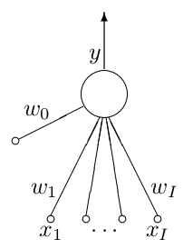from MacKay’s “Information Theory, Inference, and Learning Algorithms”

The neuron has \(I\) inputs, each \(x_i\) is weighted by \(\omega_i\) in accordance with its “importance” and an additional bias signal \(x_0\) by default feeding \(+1\) that can be deactivated by setting its weight \(\omega_0\) to 0.

The single neuron is a feed-forward device: the connections are directed from the inputs to the output \(y\) of the neuron. The output signal is decided by the Activity Rule.

Activity Rule

1. Calculate the activation \(a\) of the neurons:

\[a = \sum_{i}{\omega_i x_i}\]

2. Response \(y\) is determined through the activation function \(y=f(a)\). Some possible activation functions are:

Deterministic:

1. Linear:

\[y(a) = a\]

2. Sigmoid (logistic):

\[y(a) = \frac{1}{1+e^{-a}}\]

3. Sigmoid (tanh):

\[y(a)=\tanh(a)=\frac{e^a - e^{-a}}{e^a - e^{-a}}\]

4. Threshold step:

\[\begin{split}y(a) = \Theta(a)=\begin{cases}+1;\quad a>0\\-1;\quad a\le0\end{cases}\end{split}\]

Stochastic

1. Heat Bath (Gibbs):

\[\begin{split}y(a) = \begin{cases}+1;\quad \text{with a probability }\frac{1}{1+e^{-a}}\\-1;\quad \text{otherwise}\end{cases}\end{split}\]

2. Metropolis rule produces the output in a way that depends on the previous output state of \(y\):

   • Compute \(\Delta=ay\)

   • if \(\Delta\le0\), flip \(y\) to the other state; else flip \(y\) to the other state with a probability \(e^{-\Delta}\).

Examples

AND gate

x1	x2	y=AND
0	0	0
0	1	0
1	0	0
1	1	1

\(y(a) = \begin{cases}1;\quad a>0.5\\0;\quad\text{otherwise}\end{cases}\)

\(\omega_1 = \omega_2 = \frac{1}{2}\):

• \((0,0)\):
  \(a=\sum{\omega_i x_i}=\frac{1}{2}\cdot 0+\frac{1}{2}\cdot 0 = 0\not>0.5\quad\Rightarrow y(a)=0\)

• \((0,1)\) or \((1,0)\):
  \(a=\sum{\omega_i x_i}=\frac{1}{2}\cdot 0+\frac{1}{2}\cdot 1 = \frac{1}{2}\not>0.5\quad\Rightarrow y(a)=0\)

• \((1,1)\):
  \(a=\sum{\omega_i x_i}=\frac{1}{2}\cdot 1+\frac{1}{2}\cdot 1 = 1\gt0.5\quad\Rightarrow y(a)=1\)

NOR gate

x1	x2	x0	y=NOR
0	0	1	1
0	1	1	0
1	0	1	0
1	1	1	0

\(y(a) = \begin{cases}1;\quad a\gt0\\0;\quad\text{otherwise}\end{cases}\)

\(\omega_1 = \omega_2 = -1\), \(\omega_0 = 1\):

• \((0,0)\):
  \(a=\sum{\omega_i x_i}=0+0+1=1\gt0\quad\Rightarrow y(a) = 1\)

• \((0,1)\) or \((1,0)\):
  \(a=\sum{\omega_i x_i}=0-1+1=0\not>0\quad\Rightarrow y(a) = 0\)

• \((1,1)\):
  \(a=\sum{\omega_i x_i}=-1-1+1=-1\not>0\quad\Rightarrow y(a) = 0\)

Homework #1

1. Emulate the NOR gate without using the bias feed.

2. Propose a model for the XOR gate

3. Propose a model for the NOT gate

4. Propose a model for the NAND gate (and if you can do this, congratulations! <– do you know why? ;)

Training a single neuron as a binary classifier

Error function:

\[G(\vec{\omega}) = -\sum_{n}\left[t^{(n)}\ln{y(\vec{x}^{(n)},\vec{\omega})} + (1-t^{(n)})\ln{(1-y(\vec{x}^{(n)},\vec{\omega}))}\right]\]

This is the information content or relative entropy between the empirical probability distribution \((t^{(n)},1-t^{(n)})\) and possible probability ditribution implied by the output of the neuron \((y^{(n)},1-y^{(n)})\). The error function is equal to zero only when \(y(\vec{x}^{(n)},\vec{\omega}^{(n)}) = t^{(n)}\) for all \(n\).

Differentiate with respect to \(\vec{\omega}\):

\[\vec{g}=\frac{\partial G}{\partial \vec{\omega}}\]

\[g_j=\frac{\partial G}{\partial \omega_j}=\sum_{n=1}^{N}{-\left(t^{(n)}-y^{(n)}\right)x_j^{(n)}}\]

The error \(e^{(n)}\) is defined by:

\[e^{(n)}\equiv t^{(n)}-y^{(n)}\]

As our aim is to minimize the error by working on the weights \(\vec{\omega}\), we can proceed in two ways, differing in their learning rules:

‘Learning by example’

Activity Rule

1. Compute the activation of the neuron:

\[a = \sum_{i}{\omega_i x_i}\]

2. The output \(y\) is set as a sigmoid function of the activation:

\[y(a) = \frac{1}{1+e^{-a}}\]

This output might be viewed as the probability that the given input is in class 1 rather than class 0.

Learning Rule

The on-line gradient descent algorithm

The teacher supplies a target value \(t\in \{0,1\}\) which is the correct class for the given input. We then compute the error:

\[e=t-y\]

then adjust the weights \(\vec{\omega}\) in a direction that would reduce the magnitude of this error:

\[\Delta\omega_i = \eta e x_i\]

where \(\eta\) is the “step size” or the “learning rate”. It should be set and refined with respect to the problem at hand. Too small and the learning takes forever, too large and we miss the optimal values by far!

The batch learning algorithm

Instead of refining each weight at every step, all the weights are refined simultaneously, at the end of the batch:

1. For each input/target pair \((\vec{x}^{(n)},t^{(n)})\), compute \(y^{(n)}=y(\vec{x}^{(n)},\vec{\omega})\), where:

\[y(\vec{x}^{(n)},\vec{\omega})=\frac{1}{1+\exp{\left(-\sum_{i}{\omega_i x_i}\right)}}\]

define

\[e^{(n)}=t^{(n)}-y^{(n)}\]

and compute for each weight \(\omega_i\):

\[g_i^{(n)}=-e^{(n)}x_i^{(n)}\]

2. Then, let:

\[\Delta\omega_i = -\eta\sum_{n}{g_i^{(n)}}\]

Implementation to a code

(with the batch learning algorithm)

import numpy as np
import matplotlib.pyplot as plt
np.random.seed(371)

Define the activation function as a sigmoid

def sigmoid(v):
    v[v<-10] = -10 # Capping to prevent overflow
    return 1/(1+np.exp(-v))

Input parameters

# Input
N = 500 # Number of point-sets
xy_range = 100 # Range
N_learning_steps_max = 100000 # Number of steps for learning
eta = 0.01 # Learning rate
alpha = 0.0 # Weight decay rate

Generate the training points

# Generate N sets - x1(i),x2(i) random integers
# in the given range

x = np.random.randint(0,xy_range+1,(N,3))
x[:,2] = 1 # For the bias input

# print out the first 10
print(x[:10,:])

[[77 81  1]
 [12 91  1]
 [51 97  1]
 [62 86  1]
 [19 74  1]
 [14 87  1]
 [16 92  1]
 [72 68  1]
 [86 18  1]
 [95 95  1]]

Identify the correct classes by considering if the points are either below the diagonal or above it

# Identify the correct classes by considering
# if the points are either below the diagonal
# or above it (concerning their distances to 
# the horizontal axis)

# Seperated by diagonal (0,xy_range) - (xy_range,0)
#              <--> y = -x + xy_range
d_x = x[:,1] # point's vertical distance to x-axis
d_d = -x[:,0] + xy_range # diagonal's vert. dist. to x-axis

filter_class = d_x > d_d
t = np.zeros(N,int)
t[filter_class] = 1 # Class 1 -> above the diagonal
print(t[:10])

[1 1 1 1 0 1 1 1 1 1]

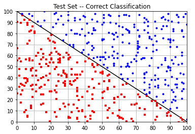
Plot the training data

# Plot the given (training) data
plt.plot([0,xy_range],[xy_range,0],"k-")
tick_step = xy_range/10

class_0 = x[t==0]
class_1 = x[t==1]
plt.plot(class_0[:,0],class_0[:,1],"rs",fillstyle="full",markersize=3)
plt.plot(class_1[:,0],class_1[:,1],"bo",fillstyle="full",markersize=3)

plt.xticks(np.arange(0,xy_range+1,tick_step))
plt.yticks(np.arange(0,xy_range+1,tick_step))
plt.grid("on")
plt.xlim(0,xy_range)
plt.ylim(0,xy_range)
plt.title("Test Set -- Correct Classification")
plt.show()

Learning Step

# Learning Step

# Initialize weights to 0
w = np.zeros(x.shape[1])

steps_so_far = 0
N_over_100 = N_learning_steps_max / 100
N_learning_steps = list(map(int,[N_over_100, 
            N_over_100*0.5, N_over_100*1.5,N_over_100*2,N_over_100*2.5,
            N_over_100*3.5, N_over_100*4,N_over_100*5,N_over_100*6,
            N_over_100*7, N_over_100*8,N_over_100*9,
                    N_over_100*10, N_over_100*20, 
                     N_over_100*30, N_over_100*40, N_over_100*50,
                     N_over_100*75, N_over_100*90, N_over_100*100
                    ]))
#print(N_learning_steps)

# Warning: the displayed "after # steps" is a little bit misleading 
# as it is actually the number of steps after the previous step.
# The real value is stored in 'steps_so_far'

for N_learning_steps_j in N_learning_steps:
    steps_so_far += N_learning_steps_j
    for i in range(N_learning_steps_j):
        a = np.dot(x,w)
        y = sigmoid(a)
        e = t - y
        g = np.dot(-x.T,e)
        w = w - eta *(g + alpha * w)
    print("Calculated Weights (after {:} steps):"\
          .format(N_learning_steps_j))
    print(w)
    y_rounded = np.round(y)
    N_misplaced = np.sum(np.abs(y_rounded-t))
    x_class0 = x[y_rounded==0]
    x_class1 = x[y_rounded==1]
    plt.plot([0,xy_range],[xy_range,0],"k-")
    tick_step = xy_range/10

    class_0 = x[y_rounded==0]
    class_1 = x[y_rounded==1]
    plt.plot(class_0[:,0],class_0[:,1]\
             ,"rs",fillstyle="full",markersize=3)
    plt.plot(class_1[:,0],class_1[:,1]\
             ,"bo",fillstyle="full",markersize=3)

    plt.xticks(np.arange(0,xy_range+1,tick_step))
    plt.yticks(np.arange(0,xy_range+1,tick_step))
    plt.grid("on")
    plt.xlim(0,xy_range)
    plt.ylim(0,xy_range)
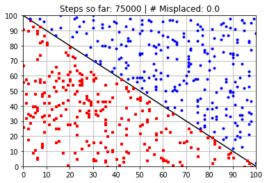
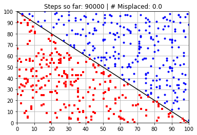
    plt.title("Steps so far: {:} | # Misplaced: {:}"\
              .format(N_learning_steps_j,N_misplaced))
    plt.show()
    print("-"*45)

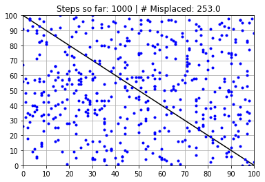
Calculated Weights (after 1000 steps):
[  90.67629591    0.99429117 -788.71877728]

---------------------------------------------
Calculated Weights (after 500 steps):
[  176.1704474    101.60306327 -1167.65515963]

---------------------------------------------

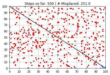
Calculated Weights (after 1500 steps):
[  188.77034033   117.19766962 -2277.04829237]

---------------------------------------------
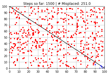
Calculated Weights (after 2000 steps):
[   43.18823521   -20.72950274 -3704.77755719]

---------------------------------------------

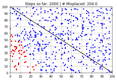
Calculated Weights (after 2500 steps):
[   40.28166291    16.01141092 -5257.57512797]

---------------------------------------------

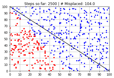
Calculated Weights (after 3500 steps):
[   58.36343559    58.39047977 -5889.29821277]

---------------------------------------------

Calculated Weights (after 4000 steps):
[   58.36493862    58.3919828  -5889.45001865]

---------------------------------------------

Calculated Weights (after 5000 steps):
[   58.36681741    58.39386159 -5889.639776  ]

---------------------------------------------

Calculated Weights (after 6000 steps):
[   58.36907195    58.39611613 -5889.86748482]

---------------------------------------------

Calculated Weights (after 7000 steps):
[   58.37170225    58.39874643 -5890.13314512]

---------------------------------------------

Calculated Weights (after 8000 steps):
[   58.37470831    58.40175249 -5890.43675688]

---------------------------------------------

Calculated Weights (after 9000 steps):
[   58.37809012    58.4051343  -5890.77832011]

---------------------------------------------

Calculated Weights (after 10000 steps):
[   58.38184769    58.40889187 -5891.15783482]

---------------------------------------------

Calculated Weights (after 20000 steps):
[   58.38936283    58.41640702 -5891.91686423]

---------------------------------------------

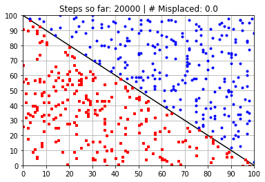
Calculated Weights (after 30000 steps):
[   58.40063555    58.42767973 -5893.05540834]

---------------------------------------------

Calculated Weights (after 40000 steps):
[   58.41566583    58.44271001 -5894.57346715]

---------------------------------------------

Calculated Weights (after 50000 steps):
[   58.43445369    58.46149787 -5896.47104067]

---------------------------------------------

Calculated Weights (after 75000 steps):
[   58.46263547    58.48967966 -5899.31740096]

---------------------------------------------

Calculated Weights (after 90000 steps):
[   58.49645362    58.5234978  -5902.73303329]

---------------------------------------------

Calculated Weights (after 100000 steps):
[   58.53402933    58.56107351 -5906.52818033]

---------------------------------------------

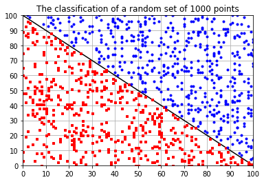
Test the learned weights against a random set

# Generate a random set
N2 = 1000
Xx = np.random.randint(0,xy_range+1,(N2,3))
Xx[:,2] = 1 # For the bias input

Xa = np.dot(Xx,w)
Xy = sigmoid(Xa)
Xy_rounded = np.round(Xy)


plt.plot([0,xy_range],[xy_range,0],"k-")
tick_step = xy_range/10

Xclass_0 = Xx[Xy_rounded==0]
Xclass_1 = Xx[Xy_rounded==1]
plt.plot(Xclass_0[:,0],Xclass_0[:,1]\
         ,"rs",fillstyle="full",markersize=3)
plt.plot(Xclass_1[:,0],Xclass_1[:,1]\
         ,"bo",fillstyle="full",markersize=3)

plt.xticks(np.arange(0,xy_range+1,tick_step))
plt.yticks(np.arange(0,xy_range+1,tick_step))
plt.grid("on")
plt.xlim(0,xy_range)
plt.ylim(0,xy_range)
plt.title("The classification of a random set of {:} points"
          .format(N2))
plt.show()

Code, combined:

"""
Single Neuron Classifier
FIZ371 Lecture Notes
21/04/2021
Emre S. Tasci
https://github.com/emresururi/FIZ371

Adapted from David MacKay's 
"Information Theory, Inference, and Learning Algorithms" book
(https://www.inference.org.uk/mackay/itila/)
"""

import numpy as np
import matplotlib.pyplot as plt
np.random.seed(371)

def sigmoid(v):
    v[v<-10] = -10 # Capping to prevent overflow
    return 1/(1+np.exp(-v))

# Input
N = 500 # Number of point-sets
xy_range = 100 # Range
N_learning_steps_max = 100000 # Number of steps for learning
eta = 0.01 # Learning rate
alpha = 0.0 # Weight decay rate

# Generate N sets - x1(i),x2(i) random integers
# in the given range

x = np.random.randint(0,xy_range+1,(N,3))
x[:,2] = 1 # For the bias input

# print out the first 10
print(x[:10,:])

# Identify the correct classes by considering
# if the points are either below the diagonal
# or above it (concerning their distances to 
# the horizontal axis)

# Seperated by diagonal (0,xy_range) - (xy_range,0)
#              <--> y = -x + xy_range
d_x = x[:,1] # point's vertical distance to x-axis
d_d = -x[:,0] + xy_range # diagonal's vert. dist. to x-axis

filter_class = d_x > d_d
t = np.zeros(N,int)
t[filter_class] = 1 # Class 1 -> above the diagonal
print(t[:10])

# Plot the given (training) data
plt.plot([0,xy_range],[xy_range,0],"k-")
tick_step = xy_range/10

class_0 = x[t==0]
class_1 = x[t==1]
plt.plot(class_0[:,0],class_0[:,1],"rs",fillstyle="full",markersize=3)
plt.plot(class_1[:,0],class_1[:,1],"bo",fillstyle="full",markersize=3)

plt.xticks(np.arange(0,xy_range+1,tick_step))
plt.yticks(np.arange(0,xy_range+1,tick_step))
plt.grid("on")
plt.xlim(0,xy_range)
plt.ylim(0,xy_range)
plt.title("Test Set -- Correct Classification")
plt.show()

# Learning Step

# Initialize weights to 0
w = np.zeros(x.shape[1])

steps_so_far = 0
N_over_100 = N_learning_steps_max / 100
N_learning_steps = list(map(int,[N_over_100, 
            N_over_100*0.5, N_over_100*1.5,N_over_100*2,N_over_100*2.5,
            N_over_100*3.5, N_over_100*4,N_over_100*5,N_over_100*6,
            N_over_100*7, N_over_100*8,N_over_100*9,
                    N_over_100*10, N_over_100*20, 
                     N_over_100*30, N_over_100*40, N_over_100*50,
                     N_over_100*75, N_over_100*90, N_over_100*100
                    ]))
#print(N_learning_steps)

# Warning: the displayed "after # steps" is a little bit misleading 
# as it is actually the number of steps after the previous step.
# The real value is stored in 'steps_so_far'

for N_learning_steps_j in N_learning_steps:
    steps_so_far += N_learning_steps_j
    for i in range(N_learning_steps_j):
        a = np.dot(x,w)
        y = sigmoid(a)
        e = t - y
        g = np.dot(-x.T,e)
        w = w - eta *(g + alpha * w)
    print("Calculated Weights (after {:} steps):"\
          .format(N_learning_steps_j))
    print(w)
    y_rounded = np.round(y)
    N_misplaced = np.sum(np.abs(y_rounded-t))
    x_class0 = x[y_rounded==0]
    x_class1 = x[y_rounded==1]
    plt.plot([0,xy_range],[xy_range,0],"k-")
    tick_step = xy_range/10

    class_0 = x[y_rounded==0]
    class_1 = x[y_rounded==1]
    plt.plot(class_0[:,0],class_0[:,1]\
             ,"rs",fillstyle="full",markersize=3)
    plt.plot(class_1[:,0],class_1[:,1]\
             ,"bo",fillstyle="full",markersize=3)

    plt.xticks(np.arange(0,xy_range+1,tick_step))
    plt.yticks(np.arange(0,xy_range+1,tick_step))
    plt.grid("on")
    plt.xlim(0,xy_range)
    plt.ylim(0,xy_range)
    plt.title("Steps so far: {:} | # Misplaced: {:}"\
              .format(N_learning_steps_j,N_misplaced))
    plt.show()
    print("-"*45)
    
# Generate a random set
N2 = 10000
Xx = np.random.randint(0,xy_range+1,(N2,3))
Xx[:,2] = 1 # For the bias input

Xa = np.dot(Xx,w)
Xy = sigmoid(Xa)
Xy_rounded = np.round(Xy)


plt.plot([0,xy_range],[xy_range,0],"k-")
tick_step = xy_range/10

Xclass_0 = Xx[Xy_rounded==0]
Xclass_1 = Xx[Xy_rounded==1]
plt.plot(Xclass_0[:,0],Xclass_0[:,1]\
         ,"rs",fillstyle="full",markersize=3)
plt.plot(Xclass_1[:,0],Xclass_1[:,1]\
         ,"bo",fillstyle="full",markersize=3)

plt.xticks(np.arange(0,xy_range+1,tick_step))
plt.yticks(np.arange(0,xy_range+1,tick_step))
plt.grid("on")
plt.xlim(0,xy_range)
plt.ylim(0,xy_range)
plt.title("The classification of a random set of {:} points"
          .format(N2))
plt.show()

Homework #2

Even though the classifier works very well with the calculated weights such as:

\[\vec{\omega}=\left(\omega_1,\omega_2,\omega_0\right)=\left( 55.65223947, 55.67928365, -5615.46740481\right)\]

these kind of high numbers don’t look very well (especially the \(\omega_0\), by the way).

Let’s try to classify once again, using the following \(\vec{\omega}\):

\[\vec{\omega}=\left(\omega_1,\omega_2,\omega_0\right)=\left( 0.01,0.01,-1.01\right)\]

and let’s blow the number of generated points to 100000 while we are at it!

import numpy as np
import matplotlib.pyplot as plt
np.random.seed(371)

def sigmoid(v):
    v[v<-10] = -10 # Capping to prevent overflow
    return 1/(1+np.exp(-v))

w = np.array([0.01,0.01,-1.01])

N2 = 100000
Xx = np.random.randint(0,xy_range+1,(N2,3))
Xx[:,2] = 1 # For the bias input

Xa = np.dot(Xx,w)
Xy = sigmoid(Xa)
Xy_rounded = np.round(Xy)


plt.plot([0,xy_range],[xy_range,0],"k-")
tick_step = xy_range/10

Xclass_0 = Xx[Xy_rounded==0]
Xclass_1 = Xx[Xy_rounded==1]
plt.plot(Xclass_0[:,0],Xclass_0[:,1]\
         ,"rs",fillstyle="full",markersize=3)
plt.plot(Xclass_1[:,0],Xclass_1[:,1]\
         ,"bo",fillstyle="full",markersize=3)

plt.xticks(np.arange(0,xy_range+1,tick_step))
plt.yticks(np.arange(0,xy_range+1,tick_step))
plt.grid("on")
plt.xlim(0,xy_range)
plt.ylim(0,xy_range)
plt.title("The classification of a random set of {:} points"
          .format(N2))
plt.show()

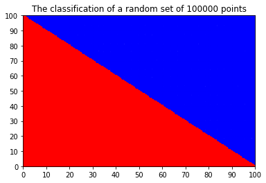
So, the question is this: How can we modify our algorithm such that instead of reaching to not so-convenient values like \(\left( 55.65223947, 55.67928365, -5615.46740481\right)\), we force it to more convenient values like \(\left( 0.01,0.01,-1.01\right)\)?

Appendix

Here is a code to help in visualizing the w-space by drawing them side by side. As it uses 3D plots, it will be much practical to run it directly as a python code.

During the execution, one can specify \((\omega_{11},\omega_{12})\) and \((\omega_{21},\omega_{22})\) along with the grid resolution seperately, e.g.,
python sigmoid_wspace.py --grid=30 --w1 -1 --w2 0 --w22 1 --w21 0 --grid=10 which will output the following:

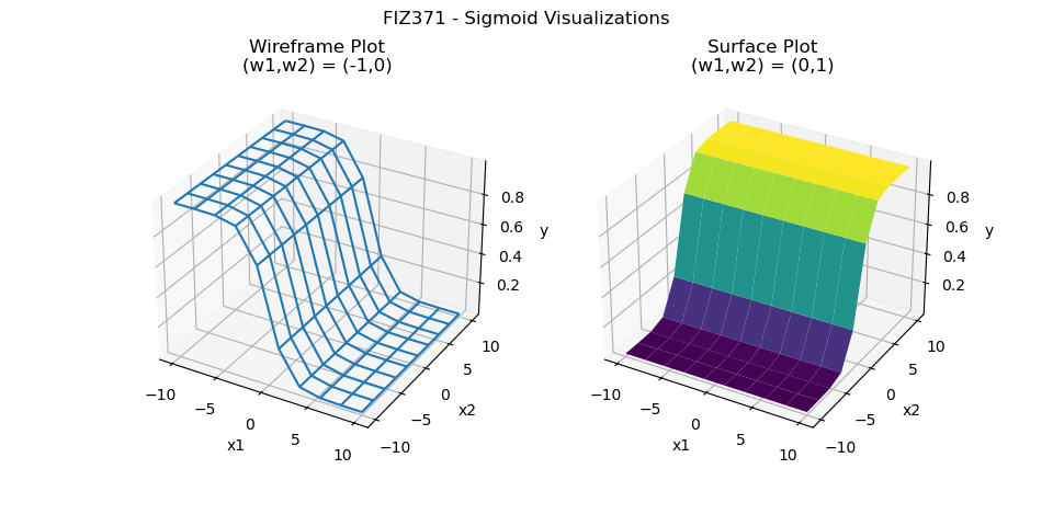
(default values: \(\omega_{*} = 1\), grid = 10)

Reference (mostly “directly copied from”)

Our usual (and wonderful) course textbook: David MacKay’s “Information Theory, Inference, and Learning Algorithms”.

History of “being beaten”

• Backgammon: 1979

• Checkers: 2007

• Chess: 1997

• Go: 2016

• Texas Hold’em Poker: 2019

• Starcraft: 2019

Places of Interest

• A Neural Network Playground : Tensorflow’s toy model for a classifier.

• The Mostly Complete Chart of Neural Networks : Almost every possible architecture models for neural networks.

Here and then…

• Using large-scale brain simulations for machine learning and A.I. : Google’s blog about how the AI learned to identify cats via neural networks (2012)

• The Physics of Fluids and Smoke (video, article)

• Neural networks news – most recent

Reading Material for the interested

• Oliver Sacks, “The Man Who Mistook His Wife For a Hat” (Karısını Şapka Sanan Adam, YKY)

• Daniel Kahneman, “Thinking, Fast and Slow” (Hızlı ve Yavaş Düşünme, Varlık)

• Iain M. Banks, “The Player of Games” (and the Culture series, in general)