Probabilities - Concept & Theory

FIZ371 - Scientific & Technical Calculations | 03/03/2021

Emre S. Tasci emre.tasci@hacettepe.edu.tr

import numpy as np

Note

The text for this lecture note is a summarized version of the 2nd chapter of David MacKay’s wonderful book “Information Theory, Pattern Recognition and Neural Networks” (which also happens to be our main source book).

Basic Distributions, Entropy and Probabilities

Ensembles

An ensemble \(X\) is a triple system: \(\left(x,A_x,P_x\right)\) where:

• \(x\): is our random variable,

• \(A_x\): is the possible value set,

• \(P_x\): is the probabilities set

\[P_x = \{p_1,p_2,\dots,p_I\}\]

\[A_x = \{a_1,a_2,\dots,a_I\}\]

\[\underbrace{P(x=a_i)}_{p(a_i)} = p_i,\;p_i\ge0,\;\sum_{a_i \in A_x}{P(x=a_i)}=1\]

Example: Frequency of letters of the alphabet.

Sub-ensemble probabilities

If \(T\) is a sub-ensemble of \(A_x\), then:

\[P(T) = P(x\in T)=\sum_{a_i \in T}{P(x=a_i)}\]

(The probabilities are added)

Joint Ensemble

\[\begin{split}\begin{array}{cl}x,y&&x\in A_x=\{a_1,\dots,a_I\},\,y\in A_y=\{b_1,\dots,b_I\}\\\text{(ordered)}&&\end{array}\end{split}\]

\(P(x,y)\): The joint probability of \(x\) and \(y\)

(Notation: \(x,y\leftrightarrow xy\))

Fig 2.2

Fig. 1 The probability distribution over the 27×27 possible bigrams xy in an English language document, The Frequently Asked Questions Manual for Linux. (Fig. 2.2 in MacKay)

Marginal Probability

\[P(x=a_i) = \sum_{y \in A_y}{P(x=a_i,y)}\]

\[P(y) = \sum_{x \in A_x}{P(x,y)}\]

Fig 2.1

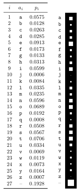
Fig. 2 Probability distribution over the 27 outcomes for a randomly selected letter in an English language document (estimated from The Frequently Asked Questions Manual for Linux ). The picture shows the probabilities by the areas of white squares. (Fig. 2.1 in MacKay)

Conditional Probability

\[P(x=a_i|y=b_j) = \frac{P(x=a_i,y=b_j)}{P(y=b_j)}\]

“Given that \(y=b_j\), what is the probability that \(x=a_i\)?”

Example: Letters in alphabet in a bigram (a word with two letters) \(xy\)

\[\underbrace{P(xy)}_{\text{Joint (Fig 1)}}: \underbrace{P(x) = P(y)}_{\text{Marginal Probabilities (Fig 2)}}\;\text{| Joint Ensemble}\]

Fig 2.3

Fig. 3 Conditional probability distributions. (a) P (y | x): Each row shows the conditional distribution of the second letter, y, given the first letter, x, in a bigram xy. (b) P (x | y): Each column shows the conditional distribution of the first letter, x, given the second letter, y. (Fig. 2.3 in MacKay)

Multiplication Rule

\[P(x,y|H) = P(x|y,H)P(y|H) = P(y|x,H)P(x,H)\]

Here, \(H\) symbolizes the “universe”, i.e., given everything else as it is.

Summation rule

\[\begin{split}\begin{align}P(y|x,H) &= \frac{P(x|y,H)P(y,H)}{P(x|H)}\\ &=\frac{P(x|y,H)P(y|H)}{\sum_{y'}{P(x|y',H)P(y'|H)}}\end{align}\end{split}\]

Independency

For \(X\) and \(Y\) to be considered independent of each other, they should satisfy:

\[P(x,y) = P(x)P(y)\leftrightarrow X\perp Y\]

Example

Jo takes a medical exam.

Variables are:

• a: Jo’s health:

  • a = 0: Jo is healthy

  • a = 1: Jo is sick

• b: Test result:

  • b = 0: Test result is negative

  • b = 1: Test result is positive

Data:

• Test is 95% reliable

• The probability that somebody at Jo’s age, status and background to be sick is 1%

Jo takes the test and the result turns out to be positive (indicating that Jo is sick). What is the probability that Jo is indeed sick?

Conditional

\[\begin{split}\begin{array}{ll}P(b=1|a=1)=0.95&&P(b=1|a=0)=0.05\\ P(b=0|a=1)=0.05&&P(b=0|a=0)=0.95\end{array}\end{split}\]

Marginal

\[P(a=1)=0.01,\;P(a=0)=0.99\]

\[\begin{split}P(a,b)=P(a)P(b|a),\\P(b=1)=P(b=1|a=1)P(a=1)+P(b=1|a=0)P(a=0)\end{split}\]

Now that we have all the probabilities we need, we can move on to the calculation:

\[\begin{split}\begin{align}P(a=1|b=1) &= \frac{P(b=1|a=1)P(a=1)}{P(b=1)}\\ &= \frac{P(b=1|a=1)P(a=1)}{P(b=1|a=1)P(a=1)+P(b=1|a=0)P(a=0)}\\ &=\frac{0.95\times 0.01}{0.95\times 0.01+0.05\times 0.99}\\ &=0.16\end{align}\end{split}\]

Hence, there is a 16% probability that Jo is indeed sick.

(0.95*0.01) / (0.95*0.01 + 0.05*0.99)

Information Content

Suppose that we want to use a coding similar to that of the Morse Coding.

Fig. 4 Source

Should we assign a single dot to “e” or “j”?

We must assign the shortest symbols (like “.” or “-”) to the most frequently used letters and long symbols (like “…” or “.-.” to the infrequently used letters to reduce the transmission time. This is reflected and calculated by the information content \(h(x)\):

\[h(x)=\log_2\frac{1}{p(x)}\]

which is measured in units of bits.

Entropy

Entropy, \(S\), in this context, is defined as the average information content:

\[S(x) = \sum_{x\in A_x}{p(x)\log_2\frac{1}{p(x)}}\]

\(\rightarrow\,S(x)\ge 0\) (only equal to 0 when \(p_i = 1\))

\(\rightarrow\) entropy is maximum when \(p\) is uniform (equal probabilities)

Expected (Average) Value

\[<x> = \sum_{x_i}{x_i p(x_i)}\]

\(\{x\} = \{1,3,3,5,7,7,7,8,9,9\}\)

\(<x> = \frac{1+3+3+5+7+7+7+8+9+9}{10}=5.9\) (“Conventional” method)

\[\begin{split}\begin{matrix}p(x_i=1)=\frac{1}{10}=0.1\\ p(x_i=2)=0\\ p(x_i=3)=\frac{2}{10}=0.2\\ p(x_i=5)=0.1\\ p(x_i=7)=0.3\\ p(x_i=8)=0.1\\ p(x_i=9)=0.2\end{matrix}\end{split}\]

\[\begin{split}\begin{align}<x>&= \sum_{x_i}{x_i p(x_i)}\\ &=1\times0.1+2\times0+3\times0.2+5\times0.1\times5+0.3\times7+0.1\times8+0.2\times9\\ &= 5.9\end{align}\end{split}\]

x = [1,3,3,5,7,7,7,8,9,9]
p = [0,0,0,0,0,0,0,0,0,0]

size = len(x)
for i in range(1,10):
    p[i] = x.count(i) / size
p

x_avg = 0
for i in range(1,10):
    x_avg += i * p[i]
print(x_avg)

Variance \((\sigma^2)\)

\[\sigma^2=<x^2>-<x>^2=\left(\sum_{x_i}{x_i^2p(x_i)}\right) \;- \left(\sum_{x_i}{x_ip(x_i)}\right)^2\]

var = 0
for i in range(1,10):
    var += i**2 * p[i]
var -= x_avg**2
print(var)

Standard Deviation \((\sigma)\)

\[\begin{split}\begin{align}\sigma &= \sqrt{\sigma^2}\\ &=\sqrt{<x^2>-<x>^2}\\ &=\sqrt{\sum_i{p_i(x_i-<x>)^2}}\end{align}\end{split}\]

x2_avg = 0
for i in range(1,10):
    x2_avg += i**2 * p[i]
print(x2_avg)

(x2_avg - x_avg**2)**0.5

var**0.5