.ipynb .md .pdf

Binder

Contents

Ordinary Differential Equations

FIZ228 - Numerical Analysis
Dr. Emre S. Tasci, Hacettepe University

import numpy as np
import matplotlib.pyplot as plt
from scipy import optimize

\(\newcommand{\diff}{\text{d}} \newcommand{\dydx}[2]{\frac{\text{d}#1}{\text{d}#2}} \newcommand{\ddydx}[2]{\frac{\text{d}^2#1}{\text{d}#2^2}} \newcommand{\pypx}[2]{\frac{\partial#1}{\partial#2}} \newcommand{\unit}[1]{\,\text{#1}}\)

A differential equation is an equation that involves one or more derivatives of a function as well as the parameters itself. If it consists of a single parameter and its function’s derivatives, we label such systems as Ordinary Differential Equations (ODEs). If more than one parameter is involved, then it is called Partial Differential Equations (PDEs).

Example

Solve the following ODE for the given boundary conditions:

\[\ddydx{x}{t}+5x=0,\quad t\in[0,20]\]

\(x(t=0) = 12,\quad x(t=20) = 40\)

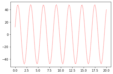
Analytical Solution

General Solution (verification)

\[\begin{split}x(t)=A\cos(\omega t + \phi), \quad \omega=\sqrt{5}\\ \ddot{x} = \ddydx{x}{t} = -\omega^2A\cos(\omega t + \phi) = -5x\\ \ddot{x} + 5x = (-5x) + 5x = 0 \end{split}\]

we also see that the period \(T\):

\[T=\frac{2\pi}{\omega}=2.81\]

Boundary Conditions

\[\begin{split}x(0) = 12 \rightarrow A\cos(\phi) = 12\quad(1)\\ x(20) = 40\rightarrow A\cos(20\omega + \phi) = A\cos(20\sqrt5+\phi)=40\quad(2)\end{split}\]

Dividing Eqn. (1) by Eqn. (2) yields:

\[\frac{\cos(\phi)}{\cos(20\sqrt5+\phi)} = \frac{12}{40}=\frac{3}{10}=0.3\]

Using the identity: \(\cos(a+b) \equiv \cos(a)\cos(b)-\sin(a)\sin(b)\), we have:

\[\frac{\cos(\phi)}{\cos(20\sqrt5)\cos(\phi)-\sin(20\sqrt5)\sin(\phi)} = 0.3\]

rearranging:

\[\begin{split}\cos(\phi) = 0.3\cos(20\sqrt5)\cos(\phi) - 0.3\sin(20\sqrt5)\sin(\phi)\\ 0.3\sin(20\sqrt5)\sin(\phi) = \left(0.3\cos(20\sqrt5)-1\right)\cos(\phi)\\ \frac{\sin(\phi)}{\cos(\phi)}=\frac{0.3\cos(20\sqrt5)-1}{0.3\sin(20\sqrt5)}\\ \phi=\tan^{-1}{\frac{0.3\cos(20\sqrt5)-1}{0.3\sin(20\sqrt5)}}\end{split}\]

phi = np.arctan2(0.3*np.cos(20*np.sqrt(5))-1,\
                 0.3*np.sin(20*np.sqrt(5)))
print(phi)

-1.3167551744556192

Now that we have \(\phi\), we can also calculate the remaining unknown, \(A\) using one of the two equations:

\[(1):\quad A = \frac{12}{\cos(\phi)}\]

A = 12/np.cos(phi)
print(A)

47.74837539488783

40/np.cos(20*5**0.5+phi)

47.74837539488792

w = np.sqrt(5)

t_a = np.linspace(0,20,200)
x_a = A*np.cos(w*t_a+phi)

plt.plot(t_a,x_a,"r:")
plt.show()

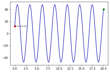
Now let’s solve it using the finite difference method.

Finite Difference Method (Derivatives Approximations)

\[y' \approx \frac{y_{i+1}-y_{i-1}}{2h}\]

\[y'' \approx \frac{y_{i-1}-2y_i+y_{i+1}}{h^2}\]

(For the detailed derivations of the approximations, refer to Programming Lecture Notes | or in our previous lecture on Interpolation (Bonus: Finite Difference Method section))

\[\ddydx{x}{t}+5x=0,\quad t\in[0,20]\]

\[x(t=0) = 12,\quad x(t=20) = 40\]

---

\[\begin{split}\ddot{x} \approx \frac{x_{i-1}-2x_i+x_{i+1}}{h^2} \\ \Rightarrow \frac{x_{i-1}-2x_i+x_{i+1}}{h^2}+5x_i=0\\ {x_{i-1}-2x_i+x_{i+1}}+5x_ih^2=0\\ x_{i-1}+(5h^2-2)x_i+x_{i+1}=0\end{split}\]

---

\[\begin{split}\begin{align*}i&=0:\quad &x_0+(5h^2-2)x_1+x_2&=0\\ i&=1:\quad &x_1+(5h^2-2)x_2+x_3&=0\\ &\;\;\vdots&\vdots\\ i&=N-3:\quad &x_{N-3}+(5h^2-2)x_{N-2}+x_{N-1}&=0 \end{align*}\end{split}\]

N = 1000
t = np.linspace(0,20,N)

h = t[1] - t[0]
h2 = h**2

x0 = 12
x_Nm1 = 40

def fun(x):
    eqns = []
    
    # i = 0
    eqns.append(x0+(5*h2-2)*x[0]+x[1])
    
    # i =  1..(N-4)
    for i in range(1,N-3):
        eqns.append(x[i-1]+(5*h2-2)*x[i]+x[i+1])
    
    # i = N-3
    eqns.append(x[N-4]+(5*h2-2)*x[N-3]+x_Nm1)
    
    return eqns

x = optimize.fsolve(fun,np.linspace(x0,x_Nm1,N-2))
x = np.insert(x,0,x0)
x = np.append(x,x_Nm1)

T = 2*np.pi/np.sqrt(5)
print("T:",T)

plt.plot(t,x,"b-")
plt.plot(20,40,"go")
plt.plot(0,x0,"ro")
plt.plot([0,T],[x0,x0],"k--")
plt.show()

T: 2.8099258924162904

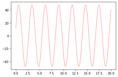
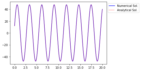
Let’s compare this analytical solution with our numerical one:

t_a = np.linspace(0,20,200)
x_a = A*np.cos(w*t+phi)

plt.plot(t,x_a,"r:")
plt.show()

t_a = np.linspace(0,20,200)
x_a = A*np.cos(w*t_a+phi)

plt.plot(t,x,"b-")
plt.plot(t_a,x_a,"r:")
plt.legend(["Numerical Sol.","Analytical Sol."],loc='upper right',\
          bbox_to_anchor=(1.35,1))
plt.show()

Example

Solve the following ODE for the given boundary conditions:

\[\begin{split}y''+y.y'+3y = \sin(x),\\ y(0) = -1, y(20) = 1.4773, x\in[0,20]\end{split}\]

We proceed by substituting the above approximations in the differential equations.

\[\begin{split}\Rightarrow y''+y.y'+3y = \sin(x) \\ \approx \frac{y_{i-1}-2y_i+y_{i+1}}{h^2} + y_i \left(\frac{y_{i+1}-y_{i-1}}{2h}\right) + 3 y_i = \sin(x_i)\\ \rightarrow y_{i-1}-2y_i+y_{i+1}+\tfrac{h}{2}y_iy_{i+1}-\tfrac{h}{2}y_iy_{i-1}+3h^2y_i=h^2\sin(x_i) \end{split}\]

Then we build N-2 equations with N-2 unknowns (unknowns being \(y_1,y_2,\dots,y_{N-2}\)):

\[\begin{split} \begin{aligned} &\begin{array}{ccc} \hline \hline \text { i } & \text { x_i } & \text { y_i } \\ \hline 0 & x_0=0 & y_0=-1 \\ 1 & x_1 & y_1 \\ \vdots & \vdots & \vdots \\ N-2 & x_{N-2} & y_{N-2}\\ N-1 & x_{N-1}=20 & y_{N-1}=1.4773\\ \hline \end{array} \end{aligned}\end{split}\]

We decide \(N\) which determines our precision since \(h=\frac{x_{N-1} - x_0}{N-1}\), i.e., the higher the number of points taken in between, the smaller the difference between consecutive points.

---

\[\begin{split}\begin{aligned} \begin{array}{ccccc} i=1 &: &\overbrace{y_0}^{-1} - 2y_1 + y_2 + \tfrac{h}{2} y_1 y_2 - \tfrac{h}{2} y_1 \overbrace{y_0}^{-1} + 3h^2 y_1 &= &h^2 \sin(x_1)\\ i=2 &: &y_1 - 2y_2 + y_3 + \tfrac{h}{2} y_2 y_3 - \tfrac{h}{2} y_2 y_1 + 3h^2 y_2 &= &h^2 \sin(x_2)\\ \vdots &: &\vdots &= &\vdots \\ i=N-2 &: &y_{N-3} - 2y_{N-2} + \underbrace{y_{N-1}}_{1.4773} + \tfrac{h}{2} y_{N-2} \underbrace{y_{N-1}}_{1.4773} - \tfrac{h}{2} y_{N-2} y_{N-3} + 3h^2 y_{N-2} &= &h^2 \sin(x_{N-1}) \end{array} \end{aligned}\end{split}\]

y_0 = -1
y_Nm1 = 1.4773

N = 250

x = np.linspace(0,20,N)
h = x[1] - x[0]
h2 = h**2

def fun(y):
    yy = np.insert(y,0,y_0)
    yy = np.append(yy,y_Nm1)
    eqns = []
    for i in range(1,N-1):
        eqns.append(yy[i-1]-2*yy[i]+yy[i+1]\
                    +h*yy[i]*yy[i+1]/2-h*yy[i]/2*yy[i-1]\
                    +3*h2*yy[i]-h2*np.sin(x[i]))
    return eqns

y = optimize.fsolve(fun,np.ones(N-2)*(y_Nm1+y_0)/2)
y = np.insert(y,0,y_0)
y = np.append(y,y_Nm1)
#y

x = np.linspace(0,20,N)
x_FD = x.copy() # For later purposes
y_FD = y.copy() # For later purposes
plt.plot(x,y,"b-")
plt.legend(["Finite Difference Method (BC)"])
plt.show()

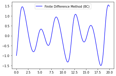
(Source: Chapra)

Example

\(y'=4e^{0.8t}-0.5y, \;y(t=0)=2\), calculate \(y\) for \(t\in[0,4]\) with a step size of \(h=1\)

Analytical solution:

\[y=\frac{4}{1.3}\left(e^{0.8t} - e^{-0.5t}\right)+2e^{-0.5t}\]

def yp(t,y):
    # The given y'(t,y) equation
    return 4*np.exp(0.8*t)-0.5*y

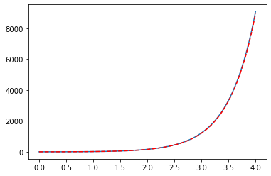
Let’s show that the given analytical solution is indeed the solution. We calculate the left side (\(y'\)) of the equation using the differentiation of the analytical solution and right side of the equation by directly plugging in the given analytical solution and compare with each other for various \(t\) values.

def dy(t):
    # y' from the analytical solution
    return 4/1.3*(0.8*np.exp(0.8*t)+0.5*np.exp(-0.5*t))-np.exp(-0.5*t)

def y_t(t):
    # true y function (analytical solution)
    return 4/1.3*(np.exp(0.8*t)-np.exp(-0.5*t))+2*np.exp(-0.5*t)

t = np.arange(0,10,0.5)
yp1 = dy(t)
yp2 = 4*np.exp(0.8*t)-0.5*y_t(t)
for tt,i,j in zip(t,yp1,yp2):
    print("{:.1f}: {:10.4f}, {:10.4f}".format(tt,i,j))

0.0:     3.0000,     3.0000
0.5:     4.0915,     4.0915
1.0:     5.8048,     5.8048
1.5:     8.4269,     8.4269
2.0:    12.3902,    12.3902
2.5:    18.3427,    18.3427
3.0:    27.2541,    27.2541
3.5:    40.5727,    40.5727
4.0:    60.4606,    60.4606
4.5:    90.1447,    90.1447
5.0:   134.4396,   134.4396
5.5:   200.5289,   200.5289
6.0:   299.1294,   299.1294
6.5:   446.2295,   446.2295
7.0:   665.6813,   665.6813
7.5:   993.0682,   993.0682
8.0:  1481.4746,  1481.4746
8.5:  2210.0933,  2210.0933
9.0:  3297.0663,  3297.0663
9.5:  4918.6407,  4918.6407

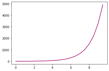
It is even easier to see that the given analytic solution is indeed the solution via plotting both sides of the equation together:

plt.plot(t,yp1,"b",t,yp2,"--r")
plt.show()

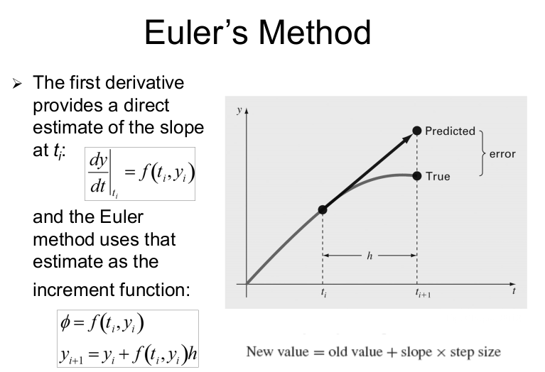
Solving the ODE using Euler Method:

t = np.arange(1,5)
h = t[1] - t[0]
y = [2]

print("{:>2s}\t{:>8s}\t{:^8s}\t{:>5s}"\
      .format("t","y_Euler","y_true","Err%"))

print("{:>2d}\t{:8.5f}\t{:8.5f}\t{:5.2f}%"\
      .format(0,y[0],y_t(0),np.abs(y_t(0)-y[0])/y_t(0)*100))
for i in t:
    slope = yp(i-1,y[i-1])
    y.append(y[i-1]+slope*h)
    print("{:>2d}\t{:8.5f}\t{:8.5f}\t{:5.2f}%"\
      .format(i,y[i],y_t(i),np.abs(y_t(i)-y[i])/y_t(i)*100))

 t	 y_Euler	 y_true 	 Err%
 0	 2.00000	 2.00000	 0.00%
 1	 5.00000	 6.19463	19.28%
 2	11.40216	14.84392	23.19%
 3	25.51321	33.67717	24.24%
 4	56.84931	75.33896	24.54%

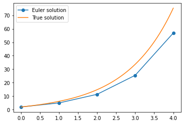
plt.plot(range(5),y,"-o",\
         np.linspace(0,4,100),y_t(np.linspace(0,4,100)),"-")
plt.legend(["Euler solution","True solution"])
plt.show()

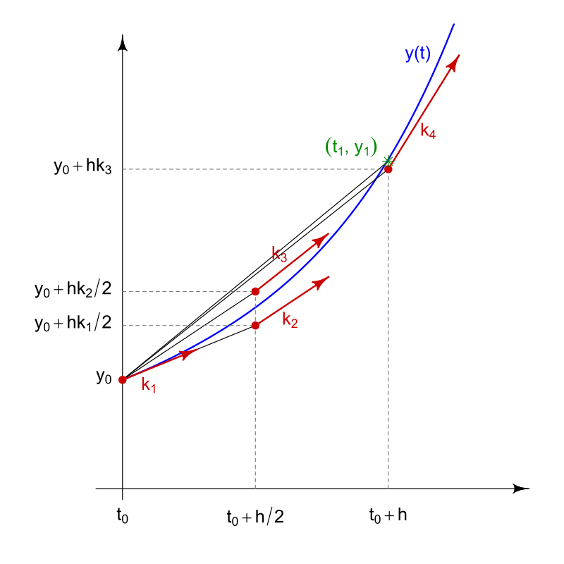
Runge-Kutta Method

(4th order Runge-Kutta: RK4)

\[y_{i+1} = y_i+\frac{1}{6}\left(k_1+2k_2+2k_3+k_4\right)h\]

where:

\[\begin{split}k_1 = f(t_i,y_i)\\ k_2= f(t_i+\tfrac{1}{2}h,y_i+\tfrac{1}{2}k_1 h)\\ k_3= f(t_i+\tfrac{1}{2}h,y_i+\tfrac{1}{2}k_2 h)\\ k_4 = f(t_i+h,y_i+k_3 h)\end{split}\]

Image: Wikipedia

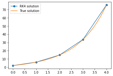
Example

\(y'=4e^{0.8t}-0.5y\), \(y(t=0)=2\), calculate \(y\) for \(t\in[0,4]\) with a step size of \(h=1\)

Analytical solution:

\[y=\frac{4}{1.3}\left(e^{0.8t} - e^{-0.5t}\right)+2e^{-0.5t}\]

def f(t,y):
    return 4*np.exp(0.8*t) - 0.5*y

def y_t(t):
    return 4/1.3*((np.exp(0.8*t)-np.exp(-0.5*t)))+2*np.exp(-0.5*t)

y = [2]
t = np.arange(5)
h = t[1]-t[0]
print("{:>2s}\t{:>8s}\t{:^8s}\t{:>5s}"\
      .format("t","y_KR4","y_true","Err%"))
for i in range(1,5):
    k1 = f(t[i-1],y[i-1])
    k2 = f(t[i-1]+0.5*h,y[i-1]+0.5*k1*h)
    k3 = f(t[i-1]+0.5*h,y[i-1]+0.5*k2*h)
    k4 = f(t[i-1]+h,y[i-1]+k3*h)
    y.append(y[i-1]+(k1+2*k2+2*k3+k4)*h/6)

for i in range(len(y)):
    print("{:>2d}\t{:8.5f}\t{:8.5f}\t{:5.2f}%"\
      .format(i,y[i],y_t(i),np.abs(y_t(i)-y[i])/y_t(i)*100))

 t	   y_KR4	 y_true 	 Err%
 0	 2.00000	 2.00000	 0.00%
 1	 6.20104	 6.19463	 0.10%
 2	14.86248	14.84392	 0.13%
 3	33.72135	33.67717	 0.13%
 4	75.43917	75.33896	 0.13%

plt.plot(range(5),y,"-o",\
         np.linspace(0,4,100),y_t(np.linspace(0,4,100)),"-")
plt.legend(["RK4 solution","True solution"])
plt.show()

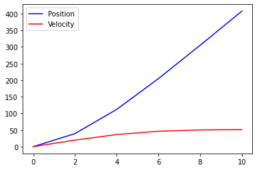
Example

Solve for the velocity and position of the free-falling bungee jumper assuming at \(t=0\), \(x=0,\;v=0\) for \(t\in[0,10]\) with a step size of 2 seconds.

Equations

\[\begin{split}v=\dydx{x}{t}\\ \dydx{v}{t} = g - \frac{C_d}{m}v^2\end{split}\]

Values: \(g=9.81\unit{ m/s}^2\), \(m=68.1 \unit{kg}\), \(C_d = 0.25 \unit{kg/m}\)

Analytical solution:

\[x(t)=\frac{\ln\left(\cosh{\sqrt{\frac{gC_d}{m}}t}\right)}{C_d/m}\]

Source: WolframAlpha

\[v(t) =\dydx{x}{t} =\sqrt{\frac{mg}{C_d}}\tanh\left(\sqrt{\frac{gC_d}{m}}t\right)\]

Source: WolframAlpha

g = 9.81 # m/s^2
m = 68.1 # kg
C_d = 0.25 # kg/m

def f(t,v):
    return g - C_d/m*v**2

N = 6

Euler

t_Euler = np.linspace(0,10,N)
h = t_Euler[1]-t_Euler[0]
x_Euler  = np.array([0])
v_Euler = np.array([0])

for ti in t_Euler[:-1]:
    v_ip1 = v_Euler[-1] + f(ti,v_Euler[-1])*h
    x_ip1  = x_Euler[-1]  + v_ip1*h
    v_Euler = np.append(v_Euler,v_ip1)
    x_Euler = np.append(x_Euler,x_ip1)

plt.plot(t_Euler,x_Euler,"-b",t_Euler,v_Euler,"-r")
plt.legend(("Position","Velocity"))
plt.show()

def x_a(t):
    # Analytical Solution
    return np.log(np.cosh(np.sqrt(g*C_d/m)*t))/(C_d/m)

def v_a(t):
    # Analytical Solution
    return np.sqrt(g*m/C_d)*np.tanh(np.sqrt(g*C_d/m)*t)

plt.plot(t_Euler,x_Euler,"-",t_Euler,x_a(t_Euler),"--r")
plt.title("x(t)")
plt.legend(["Numerical Solution","Analytical Solution"])
plt.show()

plt.plot(t_Euler,v_Euler,"-",t_Euler,v_a(t_Euler),"--r")
plt.title("v(t)")
plt.legend(["Numerical Solution","Analytical Solution"])
plt.show()

RK4

N = 6
t_aux = np.linspace(0,10,N)
h = t_aux[1]-t_aux[0]

t_RK4 = np.array([0])
x_RK4 = np.array([0])
v_RK4 = np.array([0])

for i in range(len(t_aux)-1):
    k1 = f(t[i],v_RK4[i])
    k2 = f(t[i]+0.5*h,v_RK4[i]+0.5*k1*h)
    k3 = f(t[i]+0.5*h,v_RK4[i]+0.5*k2*h)
    k4 = f(t[i]+0.5*h,v_RK4[i]+k3*h)
    v_ip1 = v_RK4[i] + (k1+2*k2+2*k3+k4)*h/6
    x_ip1 = x_RK4[i]  + v_RK4[i]*h
    
    v_RK4 = np.append(v_RK4,v_ip1)
    x_RK4 = np.append(x_RK4,x_ip1)
    t_RK4 = np.append(t_RK4,t_RK4[i]+h)

plt.plot(t_RK4,x_RK4,"-b",t_RK4,v_RK4,"-r")
plt.legend(("Position","Velocity"))
plt.show()

plt.plot(t_RK4,x_RK4,"-",t_RK4,x_a(t_RK4),"--r")
plt.title("x(t)")
plt.legend(["Numerical Solution","Analytical Solution"])
plt.show()

plt.plot(t_RK4,v_RK4,"-",t_RK4,v_a(t_RK4),"--r")
plt.title("v(t)")
plt.legend(["Numerical Solution","Analytical Solution"])
plt.show()

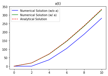
Even though the velocity fits very good, there is a discrepancy concerning the position. This is due the fact that we have derived the positions from its derivative (i.e., \(v\)):

\[ x_{i+1} = x_i + v_i h\]

where \(h\) is of course, our \(\Delta t\).

We can further refine our findings by also considering the acceleration (i.e., \(\dot v\)) and extending our formula to include that:

\[ x_{i+1} = x_i + v_i h + \frac{1}{2}\left(\frac{v_{i+1}-v_i}{h}\right) h^2\]

So, implementing this additional factor, we have:

N = 6
t_aux = np.linspace(0,10,N)
h = t_aux[1]-t_aux[0]

t_wa = np.array([0])
x_RK4_wa = np.array([0]) # This is position calculated with a
v_RK4_wa = np.array([0]) # No change in velocity's equation

for i in range(len(t_aux)-1):
    k1 = f(t[i],v_RK4_wa[i])
    k2 = f(t[i]+0.5*h,v_RK4_wa[i]+0.5*k1*h)
    k3 = f(t[i]+0.5*h,v_RK4_wa[i]+0.5*k2*h)
    k4 = f(t[i]+0.5*h,v_RK4_wa[i]+k3*h)
    v_ip1 = v_RK4_wa[i] + (k1+2*k2+2*k3+k4)*h/6
    x_wa_ip1 = x_RK4_wa[i]  + v_RK4_wa[i]*h\
               + 0.5*((v_ip1 - v_RK4_wa[i])/h)*h**2
    
    v_RK4_wa = np.append(v_RK4_wa,v_ip1)
    x_RK4_wa = np.append(x_RK4_wa,x_wa_ip1)
    t_wa = np.append(t_wa,t_wa[i]+h)

Comparing this approach with the previous one & the analytical solution:

plt.plot(t_RK4,x_RK4,"b-",t_wa,x_RK4_wa,"g-",t_RK4,x_a(t_RK4),"--r")
plt.title("x(t)")
plt.legend(["Numerical Solution (w/o a)",
            "Numerical Solution (w/ a)",
            "Analytical Solution"])
plt.show()

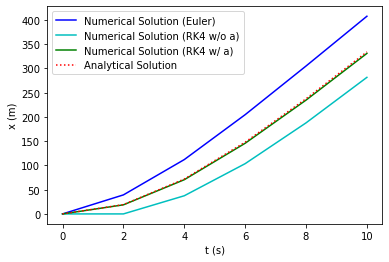
Comparison of Euler & RK4

t = np.linspace(0,10,N)

plt.plot(t_Euler,x_Euler,"-b",t_RK4,x_RK4,"-c",t_wa,x_RK4_wa,"-g",t,x_a(t),":r")
plt.xlabel("t (s)")
plt.ylabel("x (m)")
plt.legend(["Numerical Solution (Euler)",
            "Numerical Solution (RK4 w/o a)",
            "Numerical Solution (RK4 w/ a)",
            "Analytical Solution"])
plt.show()

plt.plot(t_Euler,v_Euler,"-b",t_RK4,v_RK4,"-g",t,v_a(t),":r")
plt.xlabel("t (s)")
plt.ylabel("v (m/s)")
plt.legend(["Numerical Solution (Euler)",
            "Numerical Solution (RK4)",
            "Analytical Solution"])
plt.show()

Runge-Kutta implemented in Scipy

Scipy comes with an initial value problem solver: scipy.integrate.solve_ivp(). By default, it uses the most popular version of RK, the RK45 that has been derived by blending RK4 and RK5.

It solves problems given in the form:

\[\dydx{y}{t} = f(t,y)\]

with the initial value \(y(t_0) = y_0\) and the boundaries \(t\in[t_i,t_f]\) given.

Its basic format is:

solve_ivp(f,t_range,y0)

and it returns -among other information- the t and y properties for the solution.

Let’s solve our bungee-jumper problem, this time via the built-in solver:

from scipy import integrate

# Re-define our ODE for practicality

g = 9.81 # m/s^2
m = 68.1 # kg
C_d = 0.25 # kg/m

def f_ivp(t,v):
    return g - C_d/m*v**2

Note

As the solver supports multi-variable/vector inputs, the initial value(s) should be entered as an array.

RK_solution = integrate.solve_ivp(f_ivp,[0,10],[0])
RK_solution

  message: 'The solver successfully reached the end of the integration interval.'
     nfev: 56
     njev: 0
      nlu: 0
      sol: None
   status: 0
  success: True
        t: array([0.00000000e+00, 1.00000000e-04, 1.10000000e-03, 1.11000000e-02,
       1.11100000e-01, 1.11110000e+00, 5.62593689e+00, 8.82358079e+00,
       1.00000000e+01])
 t_events: None
        y: array([[0.00000000e+00, 9.81000000e-04, 1.07909998e-02, 1.08890839e-01,
        1.08972954e+00, 1.07411772e+01, 4.07662263e+01, 4.81903652e+01,
        4.94243657e+01]])
 y_events: None

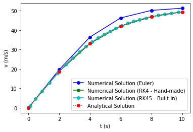
t = np.linspace(0,10,N)

ivp_t = RK_solution.t
ivp_y = RK_solution.y[0]

plt.plot(t_Euler,v_Euler,"-bo",
         t_RK4,v_RK4,"-go",
         ivp_t,ivp_y,"-co",
         t,v_a(t),":ro")
plt.xlabel("t (s)")
plt.ylabel("v (m/s)")
plt.legend(["Numerical Solution (Euler)",
            "Numerical Solution (RK4 - Hand-made)",
            "Numerical Solution (RK45 - Built-in)",
            "Analytical Solution"])
plt.show()

In the graph we see that the built-in RK45 solver determines its data points internally. We can increase the number of data considered by demanding higher accuracy via atol and rtol tolerance parameters:

RK_solution = integrate.solve_ivp(f_ivp,[0,10],[0],atol=1E-8,rtol=1E-8)

t = np.linspace(0,10,N)

ivp_t = RK_solution.t
ivp_y = RK_solution.y[0]

plt.plot(t_Euler,v_Euler,"-bo",
         t_RK4,v_RK4,"-go",
         ivp_t,ivp_y,"-co",
         t,v_a(t),":ro")
plt.xlabel("t (s)")
plt.ylabel("v (m/s)")
plt.legend(["Numerical Solution (Euler)",
            "Numerical Solution (RK4 - Hand-made)",
            "Numerical Solution (RK45 - Built-in)",
            "Analytical Solution"])
plt.show()

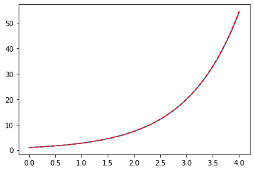
Example: 1st order ODE via Euler

\[y' = y, y(0) = 1\]

Analytical Solution: \(y(x) = e^x\)

def f(t,y):
    return y

t = np.linspace(0,4,1000)
h = t[1] - t[0]
y = np.array([1])

for tt in t[:-1]:
    y_ip1 = y[-1] + f(tt,y[-1]) * h
    #print(y_ip1)
    y = np.append(y,y_ip1)

plt.plot(t,y,"-",t,np.exp(t),"--r")
plt.show()

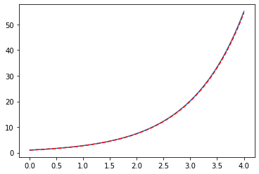
Example: 2nd order ODE via Euler \(y''=f(y)\)

\[y'' = y, y(0) = 1, y'(0) = 1\]

Analytical Solution: \(y(x) = e^x\)

def f(x,y,yp):
    # y'' = f(x,y,yp)
    return y

x = np.linspace(0,4,100)
h = x[1] - x[0]

y = np.array([1])
yp = np.array([1])

for xx in x[:-1]:
    yp_ip1 = yp[-1] + f(x[-1],y[-1],yp[-1]) *h
    yp = np.append(yp,yp_ip1)
    y_ip1 = y[-1] + yp_ip1 * h
    y = np.append(y,y_ip1)

plt.plot(x,y,"-",x,np.exp(x),"--r")
plt.show()

Example: 2nd Order ODE via Euler \(y'' = f(y,y')\)

\[y''+ y' -6y=0, y(0) = 8, y'(0)=-9\]

Analytical Solution: \(y(x) = 3e^{2x} + 5e^{-3x}\)

def f(x,y,yp):
    # y'' = f(x,y,yp)
    return 6*y - yp

x = np.linspace(0,4,1000)
h = x[1] - x[0]

y = np.array([8])
yp = np.array([-9])

for xx in x[:-1]:
    yp_ip1 = yp[-1] + f(x[-1],y[-1],yp[-1]) *h
    yp = np.append(yp,yp_ip1)
    y_ip1 = y[-1] + yp_ip1 * h
    y = np.append(y,y_ip1)

plt.plot(x,y,"-",x,3*np.exp(2*x)+5*np.exp(-3*x),"--r")
plt.show()

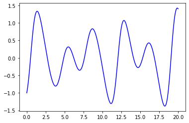
Example: 2nd Order ODE (initial conditions)

Gilberto E. Urroz

\[y''+y.y'+3y = \sin(x), y(0) = -1, y'(0) = 1, x\in[0,20]\]

def f(x,y,yp):
    # y'' = f(x,y,yp)
    return np.sin(x)-3.*y-y*yp

Euler

x = np.linspace(0,20,350)
h = x[1] - x[0]

y = np.array([-1])
yp = np.array([1])

for i in range(x.size-1):
    yp_ip1 = yp[-1] + f(x[i],y[-1],yp[-1]) *h
    yp = np.append(yp,yp_ip1)
    y_ip1 = y[-1] + yp_ip1 * h
    y = np.append(y,y_ip1)

x_Euler = x.copy()
y_Euler = y.copy()
plt.plot(x,y,"-b")
plt.show()

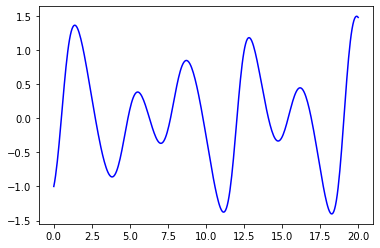
RK4

x = np.linspace(0,20,350)
h = x[1] - x[0]

y = np.array([-1])
yp = np.array([1])

for i in range(x.size-1):
    k1 = f(x[i],y[-1],yp[-1])
    k2 = f(x[i]+0.5*h,y[-1],yp[-1]+0.5*k1*h)
    k3 = f(x[i]+0.5*h,y[-1],yp[-1]+0.5*k2*h)
    k4 = f(x[i]+h,y[-1],yp[-1]+k3*h)
    yp_ip1 = yp[-1]+(k1+2*k2+2*k3+k4)*h/6
    yp = np.append(yp,yp_ip1)

    y_ip1 = y[-1] + yp_ip1 * h
    y = np.append(y,y_ip1)

x_RK = x.copy()
y_RK = y.copy()
plt.plot(x,y,"-b")
#plt.plot(x,yp,"-r")
plt.show()

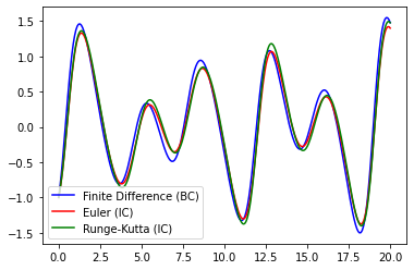
plt.plot(x_FD,y_FD,"-b")
plt.plot(x_Euler,y_Euler,"-r")
plt.plot(x_RK,y_RK,"-g")
plt.legend(["Finite Difference (BC)","Euler (IC)","Runge-Kutta (IC)"])
plt.show()

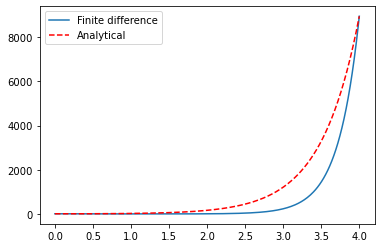
Example: 2nd Order ODE (boundary conditions, linear)

\[y'' + y' -6y=0, y(0) = 8, y(4)=8942.874,\,x\in[0,4]\]

Analytical Solution: \(y(x) = 3e^{2x} + 5e^{-3x}\)

Finite Difference Method

\[y'' \approx \frac{y_{i-1}-2y_i+y_{i+1}}{h^2}\]

\[y' \approx \frac{y_{i+1}-y_{i-1}}{h}\]

\[\begin{split}\Rightarrow y''+y'-6y = 0 \\ \approx \frac{y_{i-1}-2y_i+y_{i+1}}{h^2} + \left(\frac{y_{i+1}-y_{i-1}}{h}\right) -6 y_i = 0\end{split}\]

\[\begin{split}\rightarrow y_{i-1}-2y_i+y_{i+1}+hy_{i+1}-hy_{i-1}-6h^2y_i=0\\ (1-h)y_{i-1}-(2+6h^2)y_i+(1+h)y_{i+1} = 0\end{split}\]

---

\[\begin{split}\begin{aligned} \begin{array}{ccccc} i=1 &: &(1-h)\overbrace{y_0}^{8} - (2+6h^2)y_1 + (1+h)y_2 &= &0\\ i=2 &: &(1-h)y_1 - (2+6h^2)y_2 + (1+h)y_3 &= &0\\ \vdots &: &\vdots &= &\vdots \\ i=N-2 &: &(1-h)y_{N-3} - (2+6h^2)y_{N-2} + (1+h)\underbrace{y_{N-1}}_{8942.874} &= &0 \end{array} \end{aligned}\end{split}\]

\[\begin{split}\begin{bmatrix} -(2+6h^2) & (1+h) & 0 & 0 & 0 & \dots & 0 & 0 & 0\\ (1-h) & -(2+6h^2) & (1+h) & 0 & 0 & \dots & 0 & 0 & 0\\ 0 & (1-h) & -(2+6h^2) & (1+h) & 0 & \dots & 0 & 0 & 0\\ \vdots & \vdots & \vdots & \vdots & \vdots & \ddots & \vdots & \vdots & \vdots \\ 0 & 0 & 0 & 0 & 0 & \dots & 0 &(1-h) & -(2+6h^2) \end{bmatrix} \begin{bmatrix} y_1 \\ y_2 \\ y_3 \\ \vdots \\y_{N-2} \end{bmatrix}= \begin{bmatrix} -(1-h)y_0 \\ 0 \\ 0 \\ \vdots \\-(1+h)y_{N-1} \end{bmatrix} \end{split}\]

y_0 = 8
y_Nm1 = 8942.873991846245

N = 300
x = np.linspace(0,4,N)
h = x[1] - x[2]

ones = np.ones(N-2)
A = np.diag(ones*-(2+6*h**2))\
   +np.diag(ones*(1+h),1)[:-1,:-1]\
   +np.diag(ones*(1-h),-1)[:-1,:-1]
#print(A)

b = np.zeros((N-2,1))
b[0, 0] = -(1-h)*y_0
b[-1,0] = -(1+h)*y_Nm1
#print(b)

y = np.linalg.solve(A,b)
#print(y)
y = np.insert(y,0,y_0)
y = np.append(y,y_Nm1)
#print(y)

plt.plot(x,y,"-",x,3*np.exp(2*x)+5*np.exp(-3*x),"--r")
plt.legend(("Finite difference","Analytical"))
plt.show()

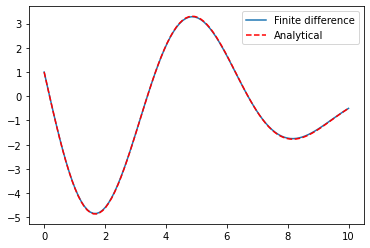
Example: 2nd Order ODE (boundary conditions, linear)

\[y'' + y -\cos(x)=0, y(0) = 1, y(10)=-0.5,\,x\in[0,10]\]

Analytical Solution: \(y(x) = (0.5x - 5.62327)\sin(x) + \cos(x)\)

\[\frac{y_{i-1}-2y_i+y_{i+1}}{h^2} + y_i -\cos(x_i)= 0\]

\[y_{i-1} - (2-h^2)y_i + y_{i+1} -h^2\cos(x_i)= 0\]

Boundary conditions:

\[\begin{split}x_0 = 0 : y_0 = 1\\x_{N-1}=10:y_{N-1} =-0.5\end{split}\]

\[\begin{split}\begin{aligned} \begin{array}{ccccc} i=1 &: &\overbrace{y_0}^{1} - (2-h^2)y_1 + y_2 &= &h^2\cos(x_1)\\ i=2 &: &y_1 - (2-h^2)y_2 + y_3 &= &h^2\cos(x_2)\\ \vdots &: &\vdots &= &\vdots \\ i=N-2 &: &y_{N-3} - (2-h^2)y_{N-2} + \underbrace{y_{N-1}}_{-0.5} &= &h^2\cos(x_{N-2}) \end{array} \end{aligned}\end{split}\]

\[\begin{split}\begin{bmatrix} -(2-h^2) & 1 & 0 & 0 & 0 & \dots & 0 & 0 & 0\\ 1 & -(2-h^2) & 1 & 0 & 0 & \dots & 0 & 0 & 0\\ 0 & 1 & -(2-h^2) & 1 & 0 & \dots & 0 & 0 & 0\\ \vdots & \vdots & \vdots & \vdots & \vdots & \ddots & \vdots & \vdots & \vdots \\ 0 & 0 & 0 & 0 & 0 & \dots & 0 &1 & -(2-h^2) \end{bmatrix} \begin{bmatrix} y_1 \\ y_2 \\ y_3 \\ \vdots \\y_{N-2} \end{bmatrix}= \begin{bmatrix} h^2\cos(x_1)-y_0 \\ h^2\cos(x_2) \\ h^2\cos(x_3) \\ \vdots \\h^2\cos(x_{N-2})-y_{N-1} \end{bmatrix} \end{split}\]

y_0 = 1
y_Nm1 = -0.5

N = 100
x = np.linspace(0,10,N)
h = x[1] - x[2]

ones = np.ones(N-2)
A = np.diag(ones*-(2-h**2))\
   +np.diag(ones,1)[:-1,:-1]\
   +np.diag(ones,-1)[:-1,:-1]
#print(A)

b =np.empty((N-2,1))
b[:,0] = h**2*np.cos(x[1:N-1])
b[0, 0] -= y_0
b[-1,0] -= y_Nm1
#print(b)

y = np.linalg.solve(A,b)
#print(y)
y = np.insert(y,0,y_0)
y = np.append(y,y_Nm1)
#print(y)

plt.plot(x,y,"-",x,(0.5*x-5.62327)*np.sin(x)+np.cos(x),"--r")
plt.legend(("Finite difference","Analytical"))
plt.show()

References

• Steven C. Chapra, “Applied Numerical Methods with MATLAB for Engineers and Scientists” 3rd Ed. McGraw Hill, 2012

• Eda Çelik Akdur, KMU231 Lecture Notes

• Gilberto E. Urroz

• Cüneyt Sert, ME310 Lecture Notes

previous

Clustering and Classification

next

Exercises & Exams