Exercise Set #3
Contents
Exercise Set #3
FIZ228 - Numerical Analysis
Dr. Emre S. Tasci, Hacettepe University
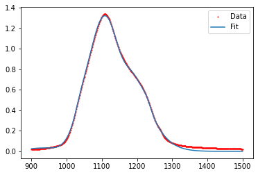
Fit the Silica FTIR data [Silica FTIR data] for the wavenumber range [900,1500] cm-1:
Using 3 Gaussians
Using 4 Gaussians
Using 5 Gaussians
Using 3 Lorentzians
Using 2 Gaussians & 2 Lorentzians
Calculate the coefficient of determination (\(r^2\)) for each fit.
Information:
A Gaussian characterized by (\(A,\mu,\sigma\)) is formulized as:
whereas, a Lorentzian characterized by (\(A,x_0,\gamma\)) is formulized as:
Hints:
Once you solve one of the items, it will be pretty straightforward to apply the same routing to the rest.
If at first you don’t get any result or error from the
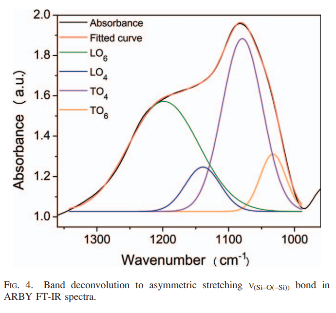
curve_fit()or any other fit function you are using, it is most likely due to a bad starting point. Trial & error is a good approach but taking a hint from Cappeletti et al.’s graph is the best one! ;) [See below]It’s always a good idea to separately plot all the components to see if the components make sense (e.g., absorbance can never take negative values!)
As an example for the last one, check the following fit of 5 Gaussians, with r2 = 0.998:
Even though it seems very good, here are its components, separately drawn:
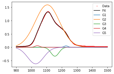
which doesn’t make any sense as G3 & G5 Gaussians indicate a negative absorption!
Cappeletti et al.’s graph
Reference & Acknowledgement
I’m indebted to Prof. Sevgi Bayarı for generously supplying the FTIR data.